Dynsmics[1] | Phase Portrait, Fixed Point, and Stability

Dynamic equations

In the previous post we covered that--

The standard form of the dynamic equation is a combination of several differential equations, all of which are first-order derivatives with respect to time and appear only on the same side of the equal sign:

$$\begin{cases} \dot z_1=\mathrm dz_1/\mathrm dt = f_1(z_1,z_2,\dots z_n) \\ \dot z_2=\mathrm dz_2/\mathrm dt = f_2(z_1,z_2,\dots z_n) \\ \dots \\ \dot z_n=\mathrm dz_n/\mathrm dt = f_n(z_1,z_2,\dots z_n) \\ \end{cases}$$

For example, let's consider a one-dimensional dynamical system

$\dot z=\frac{\mathrm dz}{\mathrm dt}=-a(z-z^*_1)(z-z^*_2)(z-z^*_3)$

Phase portrait

In addition to language and formulas, phase portraits are also often used to describe the qualitative and semi-quantitative behavior of dynamic systems, as shown below:

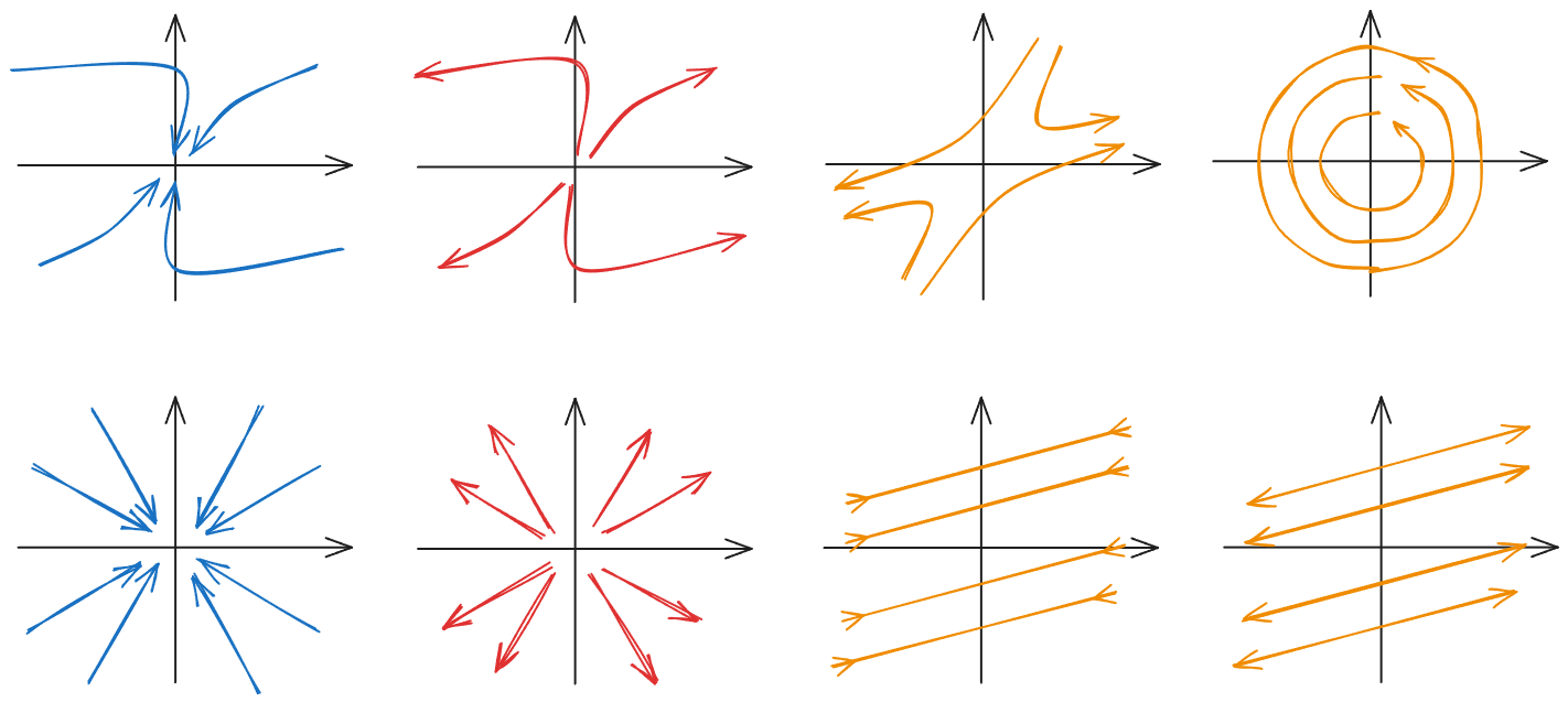
For two-dimensional dynamical systems, $f(z)$ is often annotated with arrow vector fields (e.g. using streamplot in matplotlib);

For higher-dimensional systems, it is not easy to even draw the $\vec z$ space clearly...

It is slightly humorous that as a tool for discussing time-varying functions, time does not even appear in the phase diagram (generally). The points in the phase diagram are all the possible states of the system at a certain moment. Starting from the initial state, the state points experienced by the system are connected by time, and the trajectory of the dynamic variables is drawn.

One-dimensional: generalized momentum vs. generalized coordinates

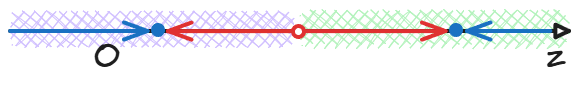
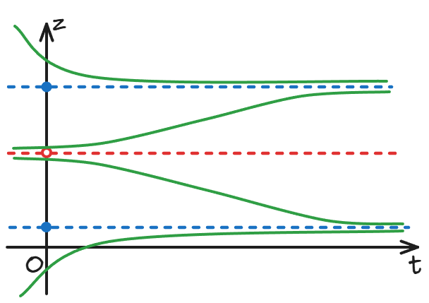
Because this is a one-dimensional dynamic system, there is still one dimension left on the paper for us to draw $f(z)$:

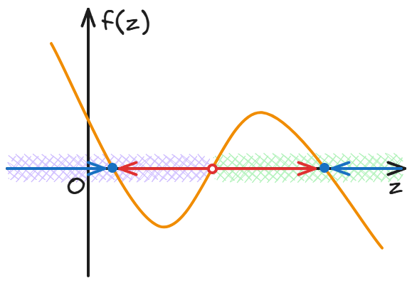
Because f(z) means the rate of change of z, or the "generalized speed", in the figure above, when f(z) is above the zero axis, the value of z will increase at the next moment, that is, it will move to the right; when f(z) is below the zero axis, z will move to the left. Therefore, the red hollow dots in the figure divide the z axis into two domains, and the points in the two domains will converge to the blue solid dots inside each domain after a long enough time.

Fixed point

The stationary point z* is the value of each physical quantity in the dynamic system that no longer changes with time once it reaches it.

$$\frac{\mathrm dz}{\mathrm dt}\bigg|_{z^*}=0$$

The stationary point $z^*$ of the one-dimensional dynamical system $\dot z = f(z)$ is the zero point of the function f.

In the previous phase diagram, the two blue solid points and the red hollow point are both stationary points.

The significance of stationary points in dynamical research should be relatively obvious:

• For the dynamical system that is currently evolving, we want to know where it will go;
• For the system that is now stationary, the value of the physical quantity is often the result of the convergence of the previous dynamical system after evolving to time $t\rarr+\infin$, which is (within the error range) the stable stationary point of the old system.

In high-dimensional dynamical systems, due to the increase in dimension, more concepts related to stationary points will be introduced, such as saddle point, nullcline, limit cycle, attractor, exotic attractor...

Stability

The "stable" stationary point in the previous article uses the concept of stability without explanation——

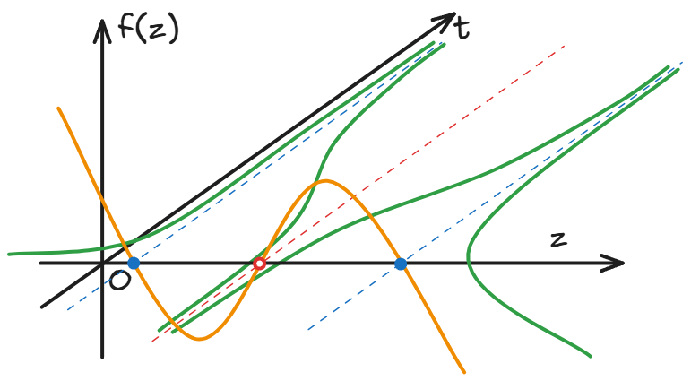
The so-called stability describes the property that when a physical quantity is in the vicinity of a stationary point, it will gradually move toward or away from the stationary point in the future.

That is, let $\eta=z-z^*$, to determine the positive or negative of $|\mathrm d \eta/\mathrm dt|$, it is often necessary to Taylor expand f near the stationary point.

In the phase diagram, it is customary to use solid points to represent stable stationary points and hollow points to represent unstable stationary points.

The stability of the one-dimensional dynamic system $\dot z = f(z)$ at the stationary point $z^*$ is generally determined by the derivative of the function f at $z^*$. When the first order is 0, the higher order should be considered. But in general, if f crosses the horizontal axis from the upper left to the lower right, the stationary point is stable; if it crosses the zero axis from the lower left to the upper right, it is unstable; if it hits the zero axis and bounces back to the original half plane, it is semi-stable.

The reason why science is not afraid of errors, in addition to the systematic error analysis tools mentioned in the previous article, is that most physical quantities are stable stationary points of dynamic systems. As long as the theory is not invalid, even if there is a gap between the current theoretical prediction and the measured value, this gap will at least not get worse and worse over time.

What's next

Linear dynamical systems