Dynamics[2] | Linear System, a Benchmark for High-Dimensional Dynamics

A linear dynamical system in n dimensions, written in matrix multiplication form:

$$\left(\begin{matrix} \dot z_1\\\dot z_2\\\vdots\\\dot z_n\end{matrix}\right)=\frac{\mathrm d}{\mathrm dt}\left(\begin{matrix}z_1\\z_2\\\vdots\\z_n\end{matrix}\right)=\left(\begin{matrix} J_{11} & J_{12} & \dots & J_{1n} \\ J_{21} & J_{22} & \dots & J_{2n} \\ \vdots & \vdots & \ddots & \vdots \\ J_{n1} & J_{n2} & \dots & J_{nn} \\ \end{matrix}\right) \left(\begin{matrix}z_1\\z_2\\\vdots\\z_n\end{matrix}\right)$$

This system of ordinary differential equations $\mathrm d\vec z/\mathrm dt=\hat J\cdot\vec z$ can be solved directly.

General solution of linear differential equations

$\hat J$ is generally a real matrix. Let $\lambda_i$ and $\vec v_i$ be the eigenvalues ​​and eigenvectors of the matrix $\hat J$.

When the eigenvalues ​​are not equal to each other

$$\vec z = \sum_i^n{c_ie^{\lambda_it}\vec v_i} = c_1e^{\lambda_1t}\vec v_1 + c_2e^{\lambda_2t}\vec v_2+\dots+c_ne^{\lambda_nt}\vec v_n$$

Where $c_i$ is a constant determined by the initial value condition, and the eigenvectors $\vec v_i$ are not necessarily** orthogonal.

Among them, an eigenvalue $\lambda_i$ may be positive, negative, complex, 0, or coincide with other eigenvalues. After a long enough evolution——

• Positive number: Each component of $\vec z$ diverges to infinity along the $\vec vi_i$ direction;
• Negative number: Each component of $\vec z$ converges to the origin along the $\vec vi_i$ direction;
• 0: Each component of $\vec z$ does not change in the $\vec vi_i$ direction, and the straight line through the origin represented by $\vec vi_i$ becomes the "stationary line" of the system
• Complex number: $\lambda$ and its conjugate $\lambda^*$ are both eigenvalues ​​of $\hat J$, and each variable spirals between this pair of eigenvectors according to Euler's formula. If the real part is positive, it spirals to infinity, and if it is negative, it spirals to the origin;
• Equal to other eigenvalues, let the multiplicity of this eigenvalue be k, then the solution of the equation becomes $\vec z = \sum_i^{n-k}{c_ie^{\lambda_it}\vec v_i}+\sum_j^kd_jt^{j-1}\vec v$

When the eigenvalues ​​are not zero, the linear system has at most one stationary point, which is the origin.

Example: 2D Linear System

In 2D, the eigenvalues ​​of the $\hat J$ matrix are given by the matrix trace $\mathrm{Tr}[\hat J]$ and the determinant $\mathrm{Det}[\hat J]$

$$\lambda_{\pm}=\frac{\mathrm{Tr}[\hat J]\pm\sqrt{\mathrm{Tr}^2[\hat J]-4\ \mathrm{Det}[\hat J]}}{2}$$

The phase portrait of the system--

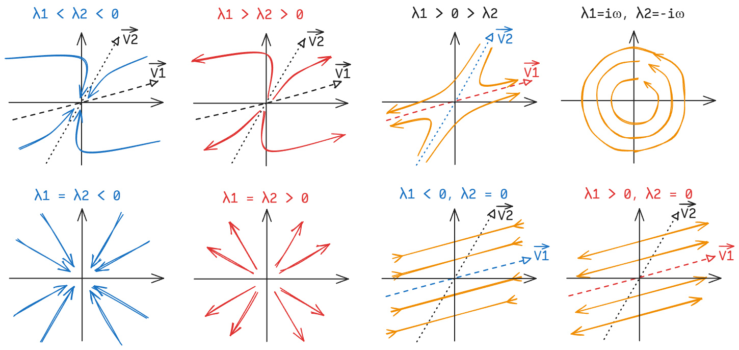
At an infinite distance from the origin, the tangent of the dynamic trajectory approaches the eigenvector with the larger absolute value of the eigenvalue.

It can be seen that in addition to stable and unstable stationary points (4 figures on the left), two-dimensional systems have several more cases than one-dimensional systems (4 figures on the right).

• The stationary point when one eigenvalue is positive and the other is negative is called a saddle point.

• When one of the eigenvalues ​​is 0, the straight line through the origin represented by the corresponding eigenvector is the fixed line of the system.

• When the two pairs of eigenvalues ​​are conjugate complex numbers, the system will have periodic phenomena, but the limit cycle will not appear until the nonlinear system.

Nullcline

There is only one f function in a one-dimensional system, and solving the stationary point only requires calculating the zero point of this function.

In high-dimensional dynamics, the zero point of $f_i$ in each dimension can be found, and the solution is an n-1-dimensional geometric structure called nullcline. In a two-dimensional dynamic system, nullclines are one-dimensional structures, that is, straight lines/curves.

On the nullcline of the kth dimension, the rate of change of the variable $z_k$ is 0, and the tangent of the trajectory of the generalized coordinates in the phase space is orthogonal to the number axis of $z_k$.

The stationary point is the common intersection of all n nullclines.

Jacobian Matrix

For a linear system represented in matrix form, the i-th row and j-th column of $\hat J$ is exactly $\partial\dot z_i/\partial z_j = \partial f_i/\partial z_j$. This partial derivative matrix between two vectors is called the Jacobian matrix $\mathbb J$.

The Jacobian matrix of a linear system has elements that are constants independent of $z_i$.

The Jacobian matrix of a nonlinear system generally has elements that are expressions with $z_i$ as variables.

The Jacobian matrix is ​​used to discuss the stability of stationary points/attractors, and its role in nonlinear systems will become more obvious in the next post.

What's next

Qualitative and semi-quantitative analysis framework for nonlinear systems